


Quick Specs
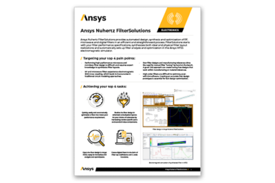
FilterSolutions provides performance specifications for every step from layout to EM optimization
Automated RF, microwave and digital filter design, synthesis and optimization in an efficient, straightforward process.
Ansys Nuhertz FilterSolutions provides automated RF, microwave and digital filter design, synthesis and optimization in an efficient, straightforward process. FilterSolutions starts with your filter performance specifications, synthesizes both lumped component and physical filter layout realizations, and automatically sets up filter analysis and optimization in the Ansys HFSS electromagnetic simulator.
FilterSolutions provides performance specifications for every step from layout to EM optimization
Ansys Nuhertz FilterSolutions dramatically speeds up the design of lumped element (surface mount) and planar filters. It also includes synthesis tools for active, switched capacitor and digital filters. The netlist of active filters can be exported in SPICE format. The digital filter synthesis module can export C-code for the generated filter.
Together with SynMatrix tool, and other unique 3D electromagnetic simulation technologies in HFSS, such as analytical derivatives and automatic adaptive meshing, these two filter solutions are making RF and microwave filter design a much smoother process that is accessible to more engineers.

JULY 2022
The Ansys 2022 R2 update release also enhances NuHertz Filter Solutions significantly, helping designers create RF filters using lumped surface mount components.
Enables optimization of planar filter designs across standard value components available from vendors. Designers of planar filters based on standard vendor parts will be able to synthesize and optimize filters as well as simulate yield analysis.
Designing high-performance microwave and mm-wave filters usually requires expert knowledge to synthesize filter layouts. A good CAE approach can create tuning-free designs that work within manufacturing or material tolerances. Creating an accurate first design prototype is essential to fast design optimization.

One of a kind solution that offers quick, easy and automatic synthesis of a filter that meets your performance requirements.
Dual user interfaces are available for simple or detailed expert filter design. If you don’t have a deep filter background, the FilterQuick interface helps you to quickly design and synthesize common filter topologies. For experts, the Filter Advanced interface provides capabilities like advanced filter shaping, pole-zero location control, custom transfer function realization, duplexer/multiplexer design and more.
Synthesizes a lumped component filter (single or double-termination) of a selected filter topology to realize your specified performance characteristics. Standard-value components may be applied, with standard (or non-standard) tolerance values for Monte-Carlo analysis. Components have ideal or finite Q, or may be based upon vendor component library models.
The Distributed Filter module synthesizes planar filter layouts on physics-accurate materials, incorporating transmission lines, vias and hybrid lumped elements. Filter layouts can performed for a variety of substrate formats, including microstrip, suspended substrate and stripline. Physical layouts (including metallization and substrate material properties) carried out quickly and accurately. Filter layouts are fully parameterized and may be seamlessly transferred to Ansys HFSS for immediate EM analysis; all geometries, materials, ports and analysis setups are automatically created. HFSS designs are fully parameterized and optimization setups are provided so you can proceed directly to design optimization to achieve filter response goals.
Some filter designs call for elimination of inductors, and active filter designs with OpAmps can sometimes be an attractive alternative. The FilterSolutions Active Filter module synthesizes filters to meet user-specified performance requirements in a wide range of active filter topologies, such as Thomas, Akerberg-Mossberg, Sallen-Key, Multiple Feedback, Leapfrog, GICs and more. Incorporate OpAmp models from your favorite vendor and include finite Q effects in your active filter designs.
Switched-Capacitor filters are zero-inductor components used in semiconductor processes where capacitors and switching transistors occupy very small spaces compared to inductors and resistors. Switched-Capacitor filters may be used to as digital filters and involve sampling circuit topologies. The Switched-Capacitor Filter module can synthesize designs in IIR and FIR realizations, as well as Bilinear, Matched-Z, Step Invariant, Modified Impulse Invariant or custom Z-transform designs.
For digital signal processing (DSP) and sampled systems, FilterSolutions takes user-specified performance specifications and a desired digital filter topology and synthesizes coefficients to produce the filter. Digital transformations are provided to Bilinear, Impulse Invariant (IIR), Step Invariant, Matched-Z and Finite Impulse Response (FIR) approximations. Filter realizations are provided in the form of the discrete transfer function, filter tap/block coefficients or as C language source code ready for incorporation into a DSP code block.
Zmatch starts with complex load definitions and synthesizes a matching network for maximum power transfer. It includes both Discrete Frequency and Broadband Match modes. Optimal matching networks are provided in lumped, distributed and hybrid realizations.
Include Bessel, Butterworth, Chebyshev I and II, Elliptic, Gaussian, Delay, Hourglass, Legendre, Matched, Raised Cosine, Tubular, Zigzag, Coupled-Resonator, Low Pass, High Pass, Band Pass, Band Stop, Diplexer, Multi-band and Cross-Coupled Folded Resonator, and Linear Phase. FilterSolutions provides an extraordinarily wide variety of useful and unique filter shapes using precision synthesis methods.
Include Lumped Translation, Inductor Translation, Stepped Impedance, Shunt Stub Resonators, Open Stub Resonators, Spaced Stubs, Dual Resonators, Spaced Dual Resonators, Parallel Edge Coupled, Hairpin, Miniature Hairpin, Ring Resonator, Interdigital and Combline. Synthesis is possible into planar components involving microstrip and inverted microstrip, stripline, symmetric and asymmetric stripline.
Include Thomas 1 and 2, Sallen & Key, Parallel, Akerberg, Multiple Feedback (MFB), GIC Biquad, GIC Ladder and Leap Frog.
Bilinear, Impulse Invariant (IIR), Matched Z, Step Invariant, FIR Approximation. FIR Filter Types: Rectangular, Bartlett, Hanning, Hamming, Blackman, Blackman-Harris, Kaiser, Dolph-Cheby, Remez, Raised Cosine, Root Raised Cosine, Cosine Filter, Sine Filter, Matched Filter and Delay Filter.
It's vital to Ansys that all users, including those with disabilities, can access our products. As such, we endeavor to follow accessibility requirements based on the US Access Board (Section 508), Web Content Accessibility Guidelines (WCAG), and the current format of the Voluntary Product Accessibility Template (VPAT).